 ...... (bohrtask.gif)
We have chosen this quatation as a motto for this work
..
..
..
..
..
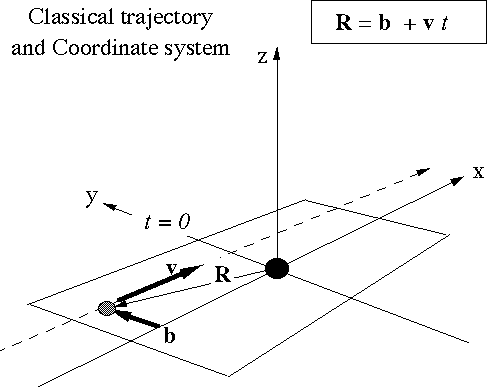
This is a picture describing the basis of the (semi) classical
collision theory. On the next picture, the plane is
rotated into the screen plane.
.. .. .. .. ..
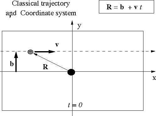
The collision plane, seen on the previous perspective drawing,
rotated into the screen plane .. .. .. .. ..
The theory: Time dependent Schroedinger equation relevant for the
collision process. The expansion in a basis set is shown.
Also shown are the kinetic energy of the electron and the two
potentials, describing the interaction with the target and the
projectile. .. .. .. .. ..
Using the expansion and evaluating projections on the basis states,
one obtains a set of coupled equations
for the coefficients as functions of time. .. .. .. .. ..
In most cases, one is satisfied by obtaining the expansion
coefficients, since the occupation probabilities (and the experimentally relevant quantities)
can be obtained from them. However, there is also the
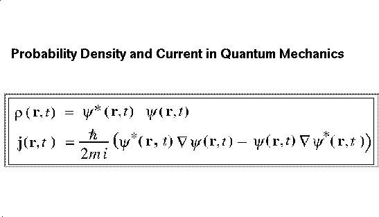
concept of probability density and probability density current.
These two quantities are defined above.
To obtain them, we must use the basis states
in "all points", i.e. on a certain mesh. This is an
additional computational effort, which cannot lead
to any comparison with experiment.
It can, however, provide cllues for understanding of the mechanisms.
.. .. .. .. ..
.. .. .. .. .. ..
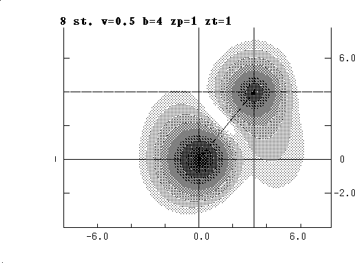
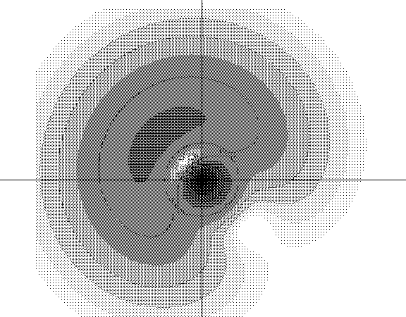
This is a plot of probability density. Each new pattern is factor 2 down, i.e.
exponential scale with steps of log 2.
.. .. .. .. ..
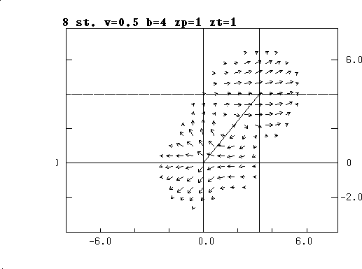
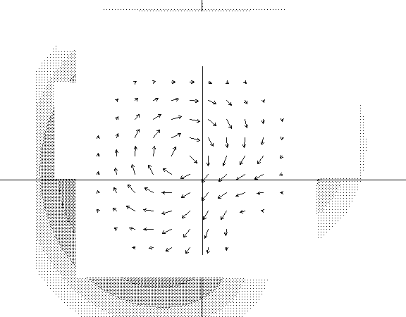
This is the corresponding probability density current. .. .. .. .. ..
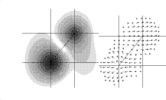
Here the two previous are compared. .. .. .. .. ..
Once more the definitions...... .. .. .. .. ..
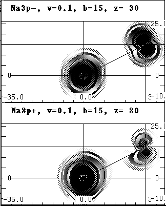
This is a cut from a movie, which one can run in task 5. This particular
picture compares two densities toowards the "end" of the collision.
The difference is in the starting condition:
The upper starts in "3p-" state, the lower in "3p+ state.
See on the next picture what does it mean in terms of currents.
.. .. .. .. ..
These are the coresponding currents "before" the collision. The picture
tells more than words and formulae.
.. .. .. .. ..
Now that collision is "finished".
Can you describe the difference? Can it be understood (or
made probable) using classical arguments?
.. .. .. .. ..
Another starting point: the states are prepared in alligned states.
What will be the difference now?
.. .. .. .. ..
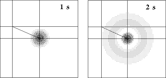
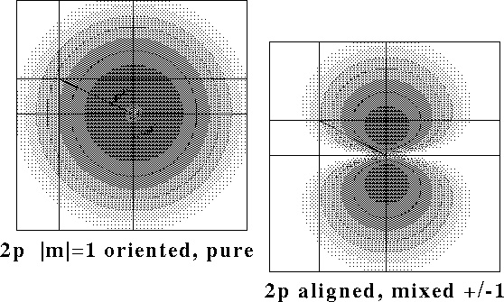
Here and in the following are pictures
of densities (and at the end 1 current),
constructed from simple amplitudes, equal to 1.
These plots show the hydrogenic
state densities. .. .. .. .. ..
Here and in the following are pictures
of densities (and at the end 1 current),
constructed from simple amplitudes, equal to 1.
These plots show the hydrogenic
state densities. .. .. .. .. ..
.. .. .. .. .. ..
BACK .... TOP ....
Links Out .....
.. .. .. .. .. .. .. .. .. .. .. ..
.. ..
Instructions .....
About The Movies .....
General Descriptions of the course
.. .. .. .. .. ..
 persp.gif
 plane.gif
 tdsep1.gif
 expand.gif
 eq1.gif
 plane.gif
 dens.gif
 curr.gif
 denscur.gif
 eq1.gif
 3pp3pm.gif
 strom1.gif
 3pp3pm2.gif
 alig.gif
 1s2s.gif
 2pand2p.gif
 1dens.gif
 1curr.gif
 atmovie.gif